bioconductor_pkgs = c("GenomicFeatures", "GenomicAlignments", "biomaRt", "Rsamtools")
cran_pkgs = "tidyverse"
devtools::source_gist("https://gist.github.com/KarenGoncalves/0db105bceff4ff69547ee25460dda978")
install_from_dif_sources(
cran_packages = cran_pkgs,
bioconductor_packages = bioconductor_pkgs
)Get read counts
Karen Cristine Goncalves, Ph.D.
2024-02-16
Data processing before R
Short read sequencing transcriptomic data (in the form of fastq files, sometimes compressed as fastq.gz) pass through the some steps before we can proceed to analysis shown in this class.
The pre-processing is typically done in servers (unix/bash language) and includes:
- Quality assessment and filtering
- IN THE ABSENCE OF A REFERENCE: Transcriptome assembly
- Read alignment/mapping
- Sorting and indexing
The things shown in this class are for alignments onto reference genomes.
Things to know
Keep track how many reads passed the quality filtering and how many were mapped.
In the case of a new assembly, you can follow steps on TrinityRNASeq wiki for transcript quantification.
Is it possible to do all the processing in R? YES
Is it worth it? …
- What you will do in R is use it to connect to another program that will do the job. So you end up using more memory (computer gets slower, takes a lot of time).
- Some programs are not available for windows, so you may install all the packages necessary just to learn that you cannot use them.
Data processing before R - detail
- Quality assessment and filtering:
- fastp (last update: 2023); fastqc (last update: 2023) followed by trimmomatic (last update: 2021)
- Creation of a reference transcriptome:
- trinity (last update: 2023); SOAPdenovo-Trans (last update: 2022); Trans-ABySS (last update: 2018); Oases (last update: 2015); Velvet (last update: 2014)
- Read alignment/mapping:
- Alignment - finds the exact origin of the reads and their differences compared to the reference (like blasting each read against a genome or transcriptome). It is slow - each alignment may take hours depending on the amount of data and size of the reference. These export SAM or BAM files, requiring indexing (step 4):
- Pseudoalignment/Mapping - hyper fast - each alignment takes minutes. They only give the genomic/transcriptomic origin of each read. These export the read count tables directly:
- If the aligner provides the result as SAM or not sorted by genomic coordinates, use
samtools viewto sort and export into sorted BAM. Then usesamtools indexto get thebaifiles.- In the end, you should have 2 files per sample/replicate:
sampleX_repY_Aligned.sortedByCoord.out.bamandsampleX_repY_Aligned.sortedByCoord.out.bam.bai
- In the end, you should have 2 files per sample/replicate:
Note that if you only want to perform differential expression analysis, GO term enrichment, etc, you do not need to perform read alignment, just mapping suffices.
Data processing before R - code example
The code below executes the 2 commands of the program STAR: the creation of the index of the genome and the alignment.
The texts within ${} are variable that should be created before hand. This ${r1/_R1.fastq} means “remove _R1.fastq” from ${r1} (like a gsub)
# Note that the adapter sequences depend on the type of sequencer
fastp -i ${raw_R1} -I ${raw_R2}\
 -o ${r1} -O ${r2}\
 --qualified_quality_phred 20\
 --unqualified_percent_limit 30\
 --adapter_sequence=TCGTCGGCAGCGTCAGATGTGTATAAGAGACAG\
 --adapter_sequence_r2=GTCTCGTGGGCTCGGAGATGTGTATAAGAGACAG\
 --cut_front --cut_front_window_size 3\
 --cut_right --cut_right_window_size 4\
 --cut_right_mean_quality 15\
 --length_required 25\
 --html $DIR/fastpReports/${r1/_R1.fastq}.html\
 --thread 8

# Let's decide if we want to map or align
MODE="align"

if [[ $MODE == "align" ]]; then
  STAR\
   --runThreadN ${NCPUS}\
   --runMode genomeGenerate\
   --genomeDir ${genomeIdxDIR}\
   --genomeFastaFiles ${genomeFastaFiles}\
   --sjdbGTFfile ${genomeGTFFile}\
   --sjdbOverhang ${readLength}

  STAR --genomeDir ${indexDIR}/\
   --runThreadN ${NCPUS} \
   --readFilesIn ${DIR}/clean_reads/${r1} ${DIR}/clean_reads/${r2} \
   --outFileNamePrefix ${DIR}/alignments/${r1/_R1.fastq}_\
   --outSAMtype BAM SortedByCoordinate \
   --outSAMunmapped Within

else
  kallisto index -i ${genomeIdxDIR} ${genomeFastaFiles}
  kallisto quant -i ${genomeIdxDIR}\
   -o ${DIR}/alignments/${r1/_R1.fastq}\
    ${DIR}/clean_reads/${r1}\
    ${DIR}/clean_reads/${r2}
fi
Installing the packages
If you use the a reference genome for which the annotation is available in Ensembl, you can create your transcript (or 5’/3’-UTR) database while you are waiting for the alignment of your reads.
For this, we need the packages “GenomicFeatures”, “GenomicAlignments”, “biomaRt”, “tidyverse”.
Setting up the scene
There are several biomarts (databases) stored in different Ensembl pages.
There is a bacteria Ensembl, but there is not a biomart for it
- Animals
- host:
"https://ensembl.org" - mart:
"ENSEMBL_MART_ENSEMBL"(currently on version 111)
- host:
- Plants
- host:
"https://plants.ensembl.org" - mart:
"plants_mart"(currently on version 58)
- host:
- Fungi
- host:
"https://fungi.ensembl.org" - mart:
"fungi_mart"(currently on version 58)
- host:
- Protists
- host:
"https://protists.ensembl.org" - mart:
"protists_mart"(currently on version 58)
- host:
There are other biomarts in the each Ensembl. You can check their names and versions with
Next thing you need is the name of the dataset.
You can check the ones available by running:
Now we have all the data we need, we set our variables:
# Edit the following based on what you need
biomart = "plants_mart"
dataset = "athaliana_eg_gene"
prefix = "ensembl_"
host = "https://plants.ensembl.org"

# The result will be saved as a .RData object, so we do not recalculate this every time.
dir = "./" # current directory
outputPath = paste0(dir, "Arabidopsis_TxDb.RData")
Then we create a Transcript DataBase (txdb) from Biomart:
# Following takes a while (a few minutes), so it is better to calculate this once than export the result
TxDb <- makeTxDbFromBiomart(biomart = biomart,
                            dataset = dataset,
                            id_prefix = prefix,
                            host = host)

# TxDb is a weird type of data, difficult to access, so we get the information on the transcripts with the function transcriptsBy
tx <- transcriptsBy(TxDb,"gene")

# Then we save the two databases into the Rdata object.
save(TxDb, tx, file = outputPath)
If you want to use the script we worked on here, just copy it below and change the section “VARIABLES” to fit your needs
###########################################
################ VARIABLES ################
###########################################
species = "Athaliana"
biomart = "plants_mart"
dataset = "athaliana_eg_gene"
prefix = "ensembl_"
host = "https://plants.ensembl.org"
dir = "./output_tables/"
outputPath = paste0(dir, species, "_TxDb.RData")

###########################################
################ Packages #################
###########################################

bioconductor_pkgs = c("GenomicFeatures", "GenomicAlignments", "biomaRt")

devtools::source_gist("https://gist.github.com/KarenGoncalves/0db105bceff4ff69547ee25460dda978")

install_from_dif_sources(
    bioconductor_packages = bioconductor_pkgs
)

###########################################
############# Create databse ##############
###########################################

TxDb <- makeTxDbFromBiomart(biomart = biomart,
                            dataset = dataset,
                            id_prefix = prefix,
                            host = host)
tx <- transcriptsBy(TxDb,"gene")

save(TxDb, tx, file = outputPath)
Getting the input files
Now that we have the .bam, .bam.bai and the transcript database RData, count the number of reads aligned to each gene.
For the example here, we will use these files (reads from Arabidopsis thaliana Col-0 GFP plants):
sapply(c("output_tables/counts", "output_tables/alignments"),
       dir.create)
site = "https://karengoncalves.github.io/Programming_classes/exampleData/"
sapply(c("subset_Col_0_GFP_1_Aligned.sortedByCoord.out.bam",
          "subset_Col_0_GFP_1_Aligned.sortedByCoord.out.bam.bai"),
       \(x) download.file(
         url = paste0(site, x),
         destfile = paste0("output_tables/alignments", x))
)
Get the counts - prepare the variables
Now that we have the files, we need to inform R where they are stored and where to put the results, in other words, prepare the variables.
- The basename here is the name of the sample_rep, without the suffix added by the aligner or samtools nor folder names (these are removed with the function
basename) - For the example, we will use a single sample, but we will use a loop so the final script can be used fo multiple samples easily
bamFiles <- paste0("/output_tables/alignments/",
                   list.files(path = "/output_tables/alignments/")
)

baiFiles <- paste0(bamFiles, ".bai")
baseNames <- gsub("_Aligned.sortedByCoord.out.bam", "",
                  basename(bamFiles))
TxDbPath <- "./output_tables/Arabidopsis_TxDb.RData"
load(TxDbPath)
outPutDir <- "./output_tables/"

# Now we load the RData
# This line tells R where the alignment files for the sample are and how much of them to read at a time
bfl <- BamFileList(bamFiles,
                   baiFiles,
                   yieldSize=200000)
Get the counts - overlaps
Summarize overlaps
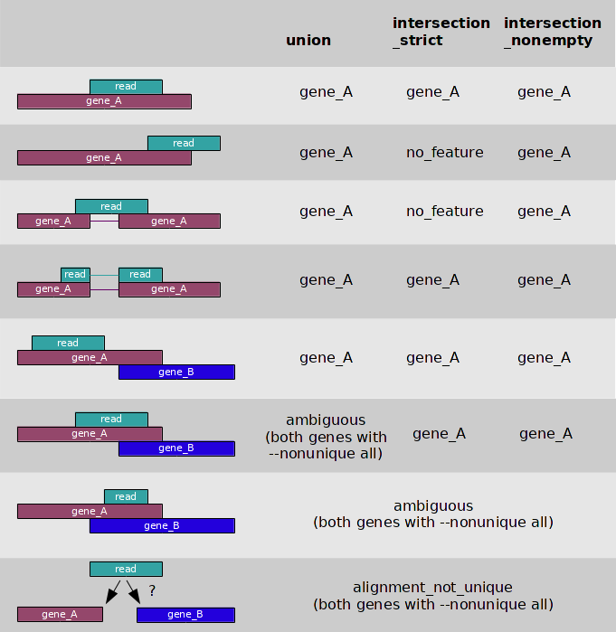
The code below uses summarizedOverlaps to count the number of alignments (bfl object) falling in each transcript (tx object, transcript database)
In this case, we have paired-end reads (singleEnd = F, fragments = T), we ignore the strand information and we use the union mode:
All the bam/bai files are analysed here. So if you have many, R will take very long to run the code. You can increase or decrease the yieldSize in the function BamFileList (previous slide) to use more/less memory and increase/decrease the speed of the code.
Get counts - export table
Now that we have the overlaps, we can get the counts.
We can check the number of reads/fragments that passed the criteria to be considered mapped using colSums. By using this function, we get the result for all datasets included in the table, without needing to explicitly type any specific sample name.
More tutorials and resources
- ARTICLE: a survey of best practices for RNA-seq data analysis
- Introduction to transcript quantification with Salmon
- End-to-end analysis - RNAseq
- RNAseq analysis in R - University of Cambridge
- RNAseq-R