Differential expression analysis
2024-03-21
The dataset
The input file is the table Arabidopsis_counts.csv.
counts = read.csv("https://karengoncalves.github.io/Programming_classes/exampleData/Arabidopsis_counts.csv",
                  header = T, row.names = 1)
This file has 12 columns (3 samples * 4 replicates) and 32833 rows (one per gene).
Samples are aerial tissue of Arabidopsis thaliana ecotype Col-0, harvested at 14 days post germination, with Basta (glyphosate) resistance gene and:
- Control: GFP under the 35S promoter
- Mlp37347 and Mlp124499: a candidate effector gene (Mlp37347 or Mlp124499 from the fungus Melampsora larici-populina) tagged with GFP under the 35S promoter
Create design table - part 1
The design table explains to R what each column is:
- Control or treatment
- Wild-type or mutant
- From place X or place Y.
- Harvested at time 0, 1, 2, 3…
Basically, you need first one column with the rows containing the same values as the column names of the count matrix.
Then, you need one (or more) columns that indicate the sample that replicate comes from.
Create design table - part 2
Note that you separate things in the columns, eg. you harvested different tissues at different time points, you would need a design table with three columns: Replicates, tissue_type and Time_point.
In this case, the genotypes of the plants is part of their name (just remove the _# to get it):
design_matrix = design_matrix %>%
  mutate(Genotype = gsub("_\\d+$", "",
                         # replace the underscore and digits at the end of the text
                         # with nothing
                         Replicates))

head(design_matrix)
Replicates Genotype
1 Control_1 Control
2 Control_2 Control
3 Control_3 Control
4 Control_4 Control
5 Mlp37347_1 Mlp37347
6 Mlp37347_2 Mlp37347Filtering read counts
Not all genes in a genome will be expressed in a study (even one with many conditions and developmental stages), since some need very specific conditions to be expressed. Check for example the gene AT1G01046 (row 5)
          Control_1 Control_2 Control_3 Control_4 Mlp37347_1 Mlp37347_2
AT1G01046         0         0         0         0          0          0
          Mlp37347_3 Mlp37347_4 Mlp124499_1 Mlp124499_2 Mlp124499_3 Mlp124499_4
AT1G01046 0 0 0 0 0 0We can clean up the data, removing genes that are not expressed ever in our experiment. In theory, genes not expressed will have read count == 0 in all samples.
Another way of filtering weakly expressed genes would be with the functions DAFS from the “KarenGoncalves/CustomSelection” package.
The function gives you the minimum expression level accepted per replicate (based on the sequencing depth), from there you can filter out the genes that are expressed at a level lower than that threshold.
You will need the count matrix and a named vector with the length of each gene.
# The first thing you do convert the read counts to TPM (transcripts per million):
tpm = Counts_to_tpm(counts=counts, featureLength=length)[[1]]

# Then you calculate the minimum expression level
cutv = DAFS(tpm=tpm) # value given as log2 TPM
# Calculate the mean minimum expression level and convert it to TPM
min_expr_level = mean(cutv) ^ 2

# Now to filter the weakly expressed genes,
# Remove the ones that are expressed below the min_expr_level
expressed_genes = apply(tpm, 1, mean) > min_expr_level
counts_filtered = countsData[, expressed_genes]
DESeq2 - main analysis
Now that you have the filtered counts matrix and the design table, you can run DESeq2 by first creating the dataset object then running the function DESeq.
Pay attention to always put your control samples at the beginning of the count matrix and the design table, as the first sample is taken as the control.
DESeq2 - note on designs
We used the design ~Genotype, which is similar to taking the expression level for each gene and compare it between the different genotypes.
It takes the first level of the factor Genotype as the control.
Because of this, the comparisons we are able to make are only Genotype_x vs Genotype_Control, we cannot compare Genotype_x against Genotype_y
Use resultsNames to see what comparisons are available
DESeq2 - note (2) on designs
If we want to make all possible pairwise comparisons, we need to add a 0 to the design function.
DESeq2 - note (3) on designs
If your samples are defined by 2 factors, say Genotype and Age (both present int the design_matrix data.frame), you can set the design to either:
~Genotype + Age- you will be able to comparegenotype1againstgenotype2, andage1againstage2, but notgenotype1_age1againstgenotype1_age2
~Genotype + Age + Genotype:Age- models the differences:- Between genotypes at the first
Agevalue - Between different time points (grouping all genotypes)
- Genotype-specific across the levels of
Age.
- Between genotypes at the first
DESeq2 - note (4) on designs
If you have a time series experiment, then you need to add a “reduced” design in the DESeq function:
Sample homogeneity
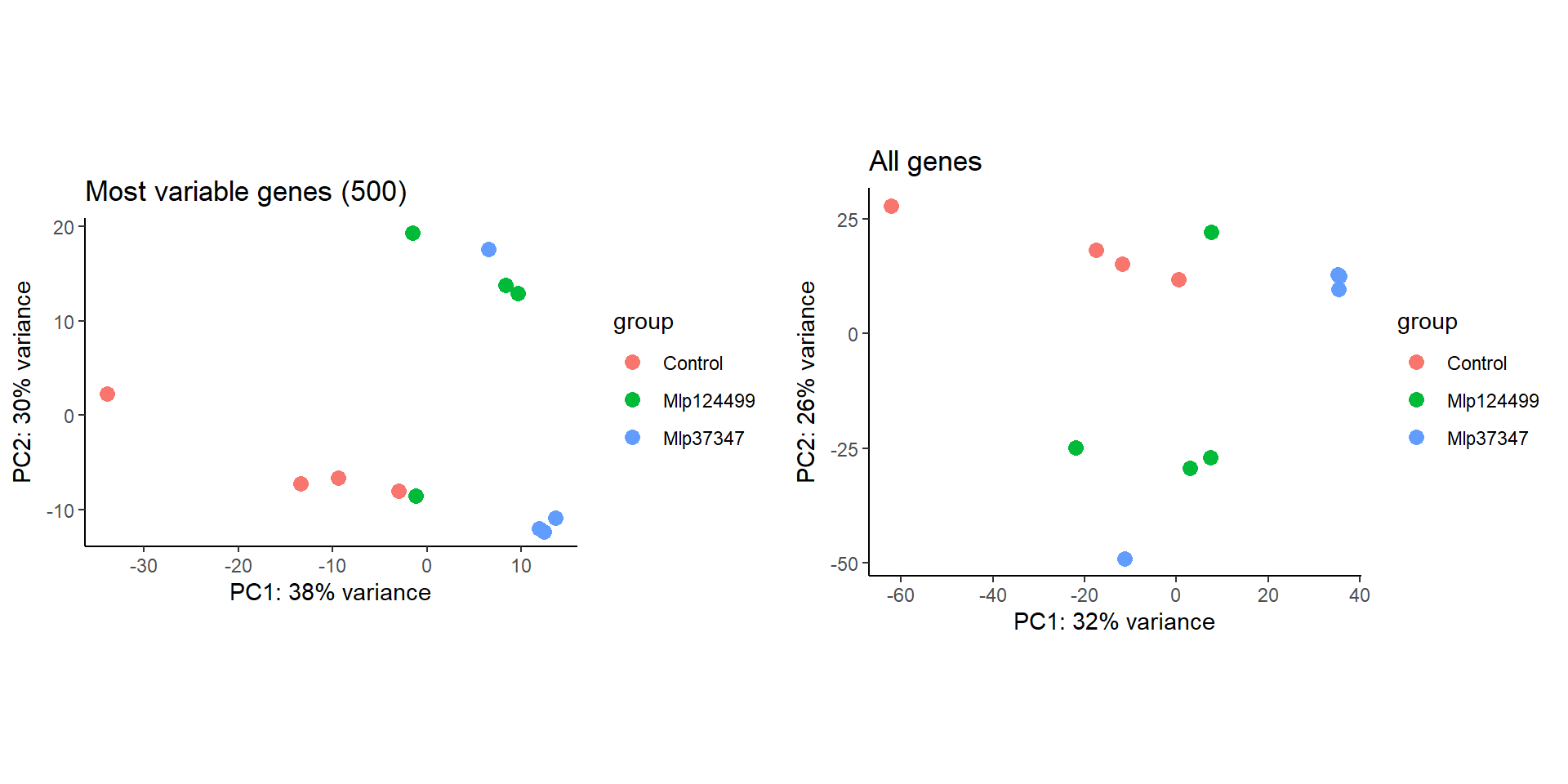
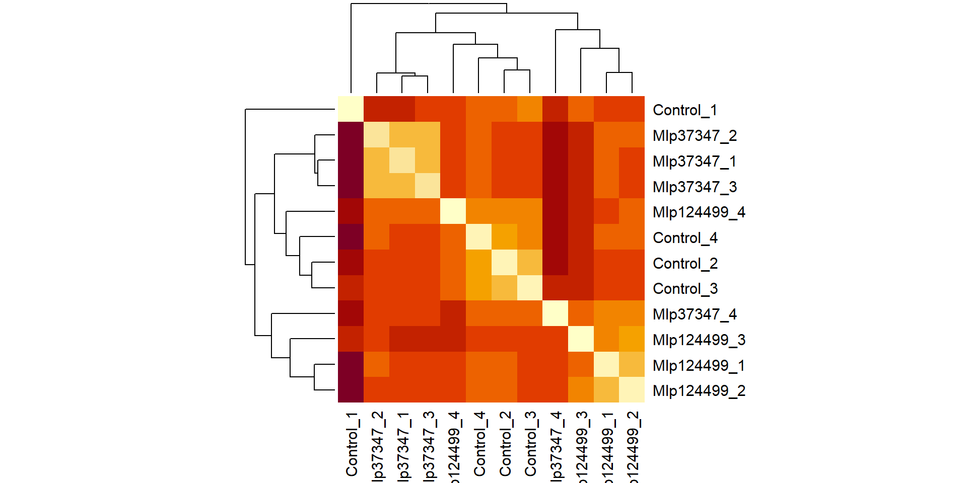
We can check the similarity of the samples and between replicates by performing one of 2 analyses: Principal Component Analysis (PCA) or Cluster Analysis.
But first, we need to get the normalized data by performing a regularized log transformation
The normalized data is stored in assays(transformed_counts)[[1]], but the PCA function from DESeq2 uses the whole rlogTransformation result
Sample homogeneity - PCA
We can either use prcomp or DESeq2::plotPCA for the PCA analysis. The normalized data is stored in assays(transformed_counts)[[1]], which is what we’d use for prcomp, but DESeq2::plotPCA uses the whole rlogTransformation result.
intgroupshould the column from design matrix used to color the replicate points in the plot
By default, plotPCA uses only the most variable genes to calculate PCA, if we want to use all genes, we need to change the ntop value
Sample homogeneity - Clustering and heatmap
Let’s calculate the difference between the samples using Euclidean distance and plot it with a heatmap and dendrogram
t() is the transpose function: shifts rows to columns and columns to rows. If we use the original data, we calculate the difference between genes.
DESeq2 results
Now the main part of the analysis is done, we use the function results to access the results and inform the type of stats you want performed.
[1] "Intercept"                     "Genotype_Mlp124499_vs_Control"
[3] "Genotype_Mlp37347_vs_Control" By setting name below, we indicate which comparison we wish to analyse, the the pAdjustMethod is the way we wish to correct the multiple tests DESeq will do (one per gene).
The result table is saved in a list, so we need to transform it to table (or tibble from tidyverse).
# Remove the first element of name_result, since it is just the intercept

results_DESeq2 <-
  lapply(name_result[-1], \(comparison) {
    results(deseq_dataset,
            name = comparison,
            pAdjustMethod = "BH")@listData %>%
      as_tibble() %>%
      mutate(
        # We need to add the gene names
        Gene_name = rownames(counts_filtered),
        # We classify the genes by deregulation
        State = case_when(
          log2FoldChange < 2 ~ "Down-regulated",
          log2FoldChange > 2 ~ "Up-regulated",
          .default = "equal"),
        # Indicate from which comparison the data comes from
        Contrast = comparison
      )
  }) %>%
  list_rbind()

head(results_DESeq2)
# A tibble: 6 × 9
baseMean log2FoldChange lfcSE stat pvalue padj Gene_name State
<dbl> <dbl> <dbl> <dbl> <dbl> <dbl> <chr> <chr>
1 73.8 -1.28 0.329 -3.89 0.0000989 0.00302 AT1G01010 Down-regul…
2 149. -0.296 0.209 -1.42 0.156 0.544 AT1G01020 Down-regul…
3 71.1 -0.709 0.248 -2.86 0.00430 0.0562 AT1G01030 Down-regul…
4 800. -0.122 0.216 -0.563 0.573 0.884 AT1G01040 Down-regul…
5 482. -0.308 0.330 -0.933 0.351 0.759 AT1G01050 Down-regul…
6 3353. -1.38 0.624 -2.21 NA NA AT1G01060 Down-regul…
# ℹ 1 more variable: Contrast <chr>Simple summary
- How many genes are deregulated in each comparison?
# A tibble: 2 × 2
# Groups:   Contrast [2]
  Contrast                          n
  <chr>                         <int>
1 Genotype_Mlp124499_vs_Control   934
2 Genotype_Mlp37347_vs_Control 1583- How many genes are up and how many down-regulated?
# A tibble: 4 × 3
# Groups:   Contrast, State [4]
  Contrast                      State              n
  <chr>                         <chr>          <int>
1 Genotype_Mlp124499_vs_Control Down-regulated   807
2 Genotype_Mlp124499_vs_Control Up-regulated     127
3 Genotype_Mlp37347_vs_Control  Down-regulated  1467
4 Genotype_Mlp37347_vs_Control  Up-regulated     116
Resources
- ARTICLES
- TUTORIALS